What Can Be Identified From a Set of Disturbance-Corrupted Input-Output Data?
We examine the problem of system identification in the presence of unknown disturbances. Available for identification are excitation signals and the resulting output responses, which may be corrupted by unknown and possibly dominating disturbances. The identification problem is subject to the following constraints: Measurements of the disturbances or disturbance-correlated signals are assumed to be unavailable. Steady-state data may not be available. Some or all disturbance frequencies may coincide with the system flexible mode frequencies. The following cases are considered:
From the available excitation and disturbance-corrupted output data, we look for the following information:
There are two solution approaches to this problem. In the explicit approach, the disturbance effect is modeled explicitly. This approach is best used in Case 1 where the disturbance profile may be exceedingly complex, Goodzeit and Phan (Jan 1997). In this case the control signal that cancels the entire disturbance effect can be determined without the need to determine the disturbance harmonic components. The explicit approach is also needed in Case 2 where basis functions are used to model the disturbance effect. The mathematical problem for Case 2 is ill-posed, therefore the solution cannot be found exactly but only approximately. Case 3 has many applications in practice, and the problem can be solved by an implicit method, where the disturbance information is implicitly present in the coefficients of an identified input-output model. These coefficients are then processed to recover the system disturbance-free dynamics and the disturbance effect, Goodzeit and Phan (1997).
For additional information on the identification problem, see also System Identification in the Presence of Unknown Disturbances and System Identification for Clear-Box Intelligent Adaptive Control.
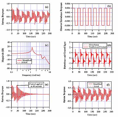
Illustration: This simulation is designed to verify various aspects of the developed system-disturbance identification theory. Consider a 3-DOF spring-mass-damper system, where a disturbance location is at the first mass, an excitation (control) input at the second mass, and the position of the third mass is used as the system output. Under known random excitation input, output data is collected in the presence of an "unknown" square-wave disturbance. Figure (a) shows the resultant system output which is clearly dominated by the square wave disturbance. This set of excitation input and disturbance-corrupted data is then presented to the identification algorithm, which correctly detects the disturbance effect as shown in Fig. (b), and correctly identifies the excitation-to-output disturbance-free dynamics as shown in Fig. (c). Figure (d) shows the feedforward control signal predicted by the identification algorithm that would negate the effect of the disturbance on the output. The unusual feedforward waveform is due to the non-collocation of the disturbance and the control input. To verify that this is the correct control signal, we run this signal through system, and observe that the controlled output indeed exhibits a free-decay response as shown in Fig. (e). We also verify that the algorithm correctly determines the steady-state contribution of the disturbance on the system output as shown in Fig. (f). All these calculations can be carried out in batch mode or recursively for real-time implementation.
An intelligent adaptive system for identification and rejection of unknown periodic disturbances is developed in this work. The system adaptively performs system identification, monitors and tracks disturbance frequencies if they are present, detects the emergence of new disturbance frequencies, predicts the effect of the each identified disturbance frequency on each system output, predicts the control energy needed to cancel each of the identified disturbance frequency for each control actuator, uses decision-making logic to determine which frequencies should be targeted and which should be ignored, and then adaptively synthesizes the necessary feedforward control to reject the selected disturbance frequencies in real-time. The formulation makes extensive use of identification to bring out otherwise hidden information about the system dynamics and the disturbance environment. This information is normally not available explicitly, and therefore bypassed in standard adaptive control approaches. This adaptive control algorithm requires only excitation input and disturbance-corrupted data to perform system-disturbance cancellation. Measurements of the disturbances or disturbance-correlated signals are assumed to be unavailable.
Illustration: This numerical study uses a fifty-second order mathematical model of the communications spacecraft shown below (artist's rendering). During an orbit adjust maneuver when thrusters are pulsed repetitively, disturbance torques excite flexible motions of the solar arrays and reflectors. To limit these motions, the adaptive system described above provides two-axis system identification and disturbance rejection. The system uses rates measured by precision gyros mounted on the spacecraft core, and sends control demands to collocated torque actuators. Actuator dynamics, sensor dynamics, and the existing rigid-body controller dynamics are incorporated into the model. The spacecraft dynamics is challenging from a system identification and control standpoint because it includes many lightly damped and closely spaced vibration modes, and several of these are nearly uncontrollable and nearly unobservable. In addition, the choice of a pulse disturbance results in significant energy in many closely spaced low-frequency harmonics (the harmonics spacing is roughly 0.524 rad/sec or 0.083 Hz). Three of the disturbance harmonics approximately coincide with the spacecraft vibration modes.

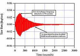
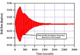
Illustration: The above spacecraft responses (yaw rate and roll rate) to the disturbance and feedforward control are shown here. The first disturbance frequency is detected after 270 seconds at which point the controller begins to react. System and disturbance identification continues, and 120 seconds later, the last (sixth)significant disturbance frequency is detected. At this point the identification process is disabled, but the disturbance rejection control continues to reduce the controlled response amplitudes further. This study demonstrates that the disturbances can be detected and canceled without producing adverse interactions between the control signals at different frequencies. Detailed description of this clear-box adaptive control formulation and extensive numerical results will be reported in Goodzeit and Phan (JVC).
Disturbance Rejection Experiments with T-Truss
T-Truss is an experimental apparatus designed to test for our "clear-box" identification and control methodology described above. The system dynamics includes approximately 10 lightly damped modes below 50 Hz, and is characteristic in many ways of real flexible space structures. The two system outputs that must be controlled are directly coupled to a disturbance source. The disturbance frequencies can be made to be coincident with the system flexible mode frequencies. The two control actuators are physically separated from the system outputs, across the length of the truss, and they must drive through the dynamics to provide control. With this non-collocated arrangement, there is no guarantee that the effect of every disturbance frequency can be canceled, or is even worth canceling given the control required. Without the capability to intelligently select frequencies for cancellation, actuator saturation, or even instability, might occur if control is blindly attempted at all disturbance frequencies present. The following experiments are performed:
The experimental results validate our techniques for analyzing models identified in the presence of unknown disturbances, illustrate the capability for selective disturbance cancellation, and show the ability of the system to provide high-accuracy control in the presence of time-varying disturbances and dynamics. The control system is consistently able to reduce the effects of the disturbances to the level of the ambient noise floor. This is significant considering that the formulation assumes very little is known about the system, only an upper bound on the effective system order and an upper bound on the number of disturbance frequencies present. Only excitation input and disturbance-corrupted output data are used, and no measurement of the disturbance input itself is assumed. See Goodzeit, Phan, and Frueh (to appear) for a detailed report of these experiments.
Illustration: The following result illustrates why our system-disturbance identification technique is needed. From system theory, it is known that uncontrollable modes do not contribute the system input-output map; hence the presence of harmonic disturbances in the output data should not corrupt the identified input-output transfer function (i.e., the disturbance "modes" would appear as perfectly canceling pole and zero pairs). In practice, this cancellation is not complete, and the identified input-output map may be severely corrupted by such disturbances. The left figure on shows the reference pulse response identified with disturbance-free input-output data. The right figure shows the same identified with disturbance-corrupted data. In theory the two should be identical, but in practice they are not. Indeed, the unknown disturbances can significantly corrupt the identified dynamics model such that it is unusable without additional processing.
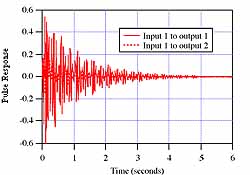
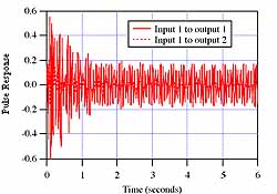
Illustration: Despite this corruption, using our developed system-disturbance identification technique, it is possible to accurately separate the effects of the system dynamics and disturbances to obtain a high-fidelity dynamics model and disturbance information. This is accomplished by identifying and evaluating the model's constituent modes, and observing how they change with increasing over-parametrization. From this analysis it is then possible to arrive at a full or reduced-order model of sufficient accuracy for control applications (by selective modal truncation). The following figure shows an overlay of the transfer function identified with disturbance-corrupted data against that identified with disturbance-free data.
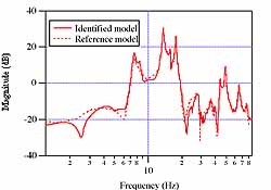
Illustration: In this experiment, random excitation is applied to the proof-mass control actuators located at one end of the structure. Acceleration measurements are made at one node on the other end of the structure. An "unknown" disturbance is injected into the structure while data is being collected for identification. This disturbance signal consists of 10 harmonic components, 5 of them are (by design) coincident with the system flexible modes. Only excitation input data and disturbance-corrupted output data are used for system identification which successfully recovers correctly the system disturbance-free input-output dynamics by separating overlapping system and "disturbance modes". All 10 disturbance frequencies are also correctly identified. In addition, the identification technique computes the contribution of each disturbance frequency on each of the two output accelerometers, and the control effort needed at each of the two control actuators to cancel each of these disturbance frequencies. All this information is obtained by identification alone before any actual control is applied. A table of identification results is provided in System Identification for Clear-Box Intelligent Adaptive Control. From this table it can be decided which disturbance frequencies should be targeted for cancellation to account for limited control resources. The left figure shows the controlled system response when 5 disturbance frequencies are selected for rejection. The right figure shows the needed control input signals at each of the two actuators. If we blindly attempt to cancel all 10 disturbance frequencies, the actuators will quickly saturate, resulting possible instability.
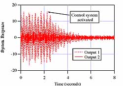
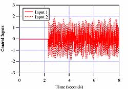
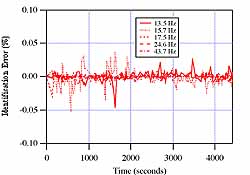
Illustration: This experiment demonstrates that the control formulation can handle unknown disturbances with time-varying frequencies. In this case the disturbance includes five frequencies initially at 13.5, 15.7, 17.5, 24.6, and 43.7 Hz, that coincide with the lightly damped system modes at these same frequencies. The disturbance frequencies are varied over time, and occasionally they cross over the system flexible mode frequencies during the experiment. The adaptive identification system tracks the frequency variation (left figure) and the adaptive control system continuously updates the control coefficients to maintain continuous disturbance rejection. The right figure shows the response amplitude measured in terms of its standard deviations over time.
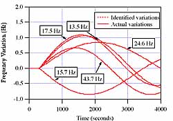
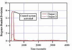
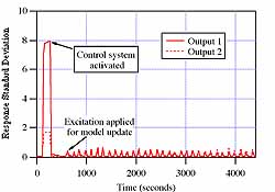
Illustration: This experiment shows how the adaptive system performs in the presence of time variations in both the disturbance frequencies and system dynamics. As in the previous experiment, the disturbance frequencies are varied over time. The dynamics time variation is accomplished by transforming the acceleration signals to a coordinate frame that rotates 90 degrees in one hour (this rate of variation is six times larger than that typically encountered for a geosynchronous spacecraft). At the end of the experiment the inputs to the control system are effectively switched, acceleration signal 1 is now acceleration signal 2, and vice versa. The tracking errors of the time-varying disturbance frequencies are shown in the left figure. The right figure shows the adaptive control system performance. To keep track of the time-varying dynamics, the system must be periodically excited to collect data for identification. The right figure shows how the system performance is degraded due to this excitation. It is verified here that this cost is small when compared to the cost of doing nothing (where the response amplitude would rise to a much higher level).