State Space System Identification

Much of system identification theory has been developed by the adaptive estimation and control community. As a result, the natural emphasis has been on input-output models. However, modern control is built up on state-space models, for which well-known results such as Kalman filtering, LQR, LQG, etc. have become defining hallmarks of the field. The state-space approach provides insights into the control problem that may be more difficult to see from the input-output perspective. It is indisputable that tremendous understanding has been gained by going from the input-output transfer function approach of classical control to state-space approach of modern control. With this insight we seek an analogous development in system identification to achieve a similar gain by going from input-output model identification to state-space system identification. In state-space identification, however, not all the state variables can be assumed to be measurable, and as in the case of input-output identification, we still must work with input-output data and input-output models. Thus for state-space identification to succeed, new understanding of how various input-output models and state-space models are connected is crucial. One may argue that it is always possible to convert an identified input-output model into a state-space model, and thus, in a sense, input-output identification and state-space identification are equivalent. This argument, although strictly correct, would preclude the development of a large number of useful identification results that one may obtain if the state-space model is a starting point of the theoretical consideration. Another benefit of state-space identification is that these results will naturally allow system identification to be unified on the same level with modern control theory, as opposed to remaining a related but somewhat isolated relative. For example, one can identify a state-space model and an optimal observer gain (e.g., a Kalman filter gain) simultaneously from a set of noise contaminated input-output data for use in a modern state-feedback control system. This is possible when one understands how the state-space model parameters and the Kalman filter gain are interwined in the coefficients of a certain input-output model so that the reverse process of extracting the state-space model and the Kalman filter gain can be carried out. Finally, state-space system identification will also help making modern control more attractive to be applied in practice.

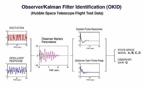
Observer/Kalman Filter Identification (OKID)

Given a set of input-output data which may be contaminated by process and measurement noise, we find the system state-space model A,B,C,D and an associated observer gain M which is optimal with respect to the process and measurement noise in the data. Under conditions normally associated with a Kalman filter, it can be shown that the identified observer gain converges to the steady-state Kalman filter gain as the length of the data record and the order of the identified input-output model increase. The identified Kalman filter gain is the one associated with the unknown process and measurement noise statistics embedded in the input-output data. This solution is obtained by understanding how the state-space model parameters and the observer/Kalman filter gain are interwined in the coefficients of a certain input-output model so that the reverse process of extracting the state-space model and the Kalman filter gain can be carried out. With this technique, the nonlinear problem of estimating of the system state together with its state-space model parameters is avoided. Instead the nonlinear problem is deferred to the final step where one takes advantage of the well-developed realization theory for which an exact and closed-form solution of the nonlinear realization problem has already been found. This algorithm is implemented as a easy-to-use function in a Matlab-based OKID toolbox. The user supplies a set of sampled input-output data, the sampling interval, the number of inputs and outputs, and a guess on an upper bound on the order of the state-space model to be identified. The OKID function returns an identified state-space model A,B,C,D together an associated observer/Kalman filter gain M. The system true or effective order will also be recovered as part of the identification process. As mentioned, this is a closed-form solution and no nonlinear iteration is involved. See Juang et al. (1993), Phan et al. (1993, 1992), and Chen et al. (1992) for more details. OKID with residual whitening is presented in Phan et al. (1995).

Illustration: The following chart illustrates the key steps involved in OKID. Shown are actual experimental excitation and response data collected from the Hubble Space Telescope in orbit. From this set of data, a special set parameters called Observer Markov Parameters, which are linearly related to input-output data, are computed. The needed information (the system state-space model and an associated observer gain) are scrambled non-linearly in these Observer Markov Parameters. However, the Observer Markov Parameters can be "unscrambled" to obtain the desired model and observer gain analytically without having to resort to any kind of non-linear iterative solution technique. The final outcome of OKID is a state-space model for the system, and an observer gain which is optimal with respect to the process and measurement noise embedded in the input-output data. The identified state-space model and observer gain are now ready to be used in the design an observer-based state feedback modern control system.

Observer/Controller Identification (OCID)

It extends the observer identification method of OKID to closed-loop system identification. The goal is to extract the system open-loop dynamics from closed-loop data. We first consider the case where the closed-loop system has an observer-based state-feedback controller. The method, referred to as OCID for Observer/Controller Identification, identifies the system open-loop state-space model, an associated observer gain, and a state feedback controller gain of the existing closed-loop control system. The user supplies closed-loop excitation data and control signal. This method was applied successfully to extract open-loop unstable flutter modes of an actively controlled aircraft wing in a wind tunnel at NASA Langley Research Center. As in the case of OKID, this is a closed-form solution and no nonlinear iteration is involved. See Juang and Phan (1994) for more details.

When the closed-loop system has a dynamic output feedback controller instead of an observer-based state-feedback controller, the open-loop system can also be identified as well using the observer identification framework. In this case the user supplies closed-loop excitation data and the existing dynamic output feedback controller gains, the algorithm returns the system open-loop state-space model. The system true or effective order will also be recovered as part of the identification process. See Phan et al. (1994) for more details.

Illustration: The following chart illustrates the key steps involved in OCID. Shown in this illustration are actual experimental data collected from an actively controlled aircraft wing in a wind tunnel at NASA Langley Research Center. Data was collected when the aircraft wing was under closed-loop control to suppress flutter (instability) at a certain aerodynamic condition. From this set of data we are interested in recovering the system open-loop dynamics. In other words, although it was not possible to perform open-loop system identification (because of the instability) we would like to extract from closed-loop data the system behavior if the controller were to be removed. From closed-loop data, a special set parameters called Observer/Controller Markov Parameters are computed. From this set of parameters, the system unstable open-loop dynamics is recovered (notice the pulse response with growing amplitude). In addition to recovering the system open-loop state space model, OCID also identifies the system existing state feedback controller gain, and an optimal observer gain associated with the process and measurement noise embedded in the experimental data.

New Connection between Input-Output and State-Space Models

Understanding how the state-space model coefficients relate to input-output data is very important for state-space identification. Traditionally, this connection is explained via well-known observable and controllable canonical realizations. Recently, however, it is established that the connection between the two model structures can be explained in terms of a new set of parameters called observer Markov parameters. This connection allows new ways of performing state-space system identification from input-output data. Even more recently, the observer Markov parameter connection can be generalized further in the context of a generalized Cayley-Hamilton theorem. This latter connection extends state-space system identification problem to state-space predictive control.

• Observer Markov Parameters: These parameters generalize the standard system Markov parameters by incorporating information of an associated observer. In the deterministic case, the observer Markov parameters subsume a state-space model and a deadbeat observer gain. In the stochastic case, the observer Markov parameters contain information of an observer such as a Kalman filter. The observer Markov parameters can be identified directly from input-output data. One can extract from the identified observer Markov parameters not only a state-space model of the system, but also an associated optimal observer gain for use in modern state-space based feedback control. See Phan, Juang, and Longman (1997) for a tutorial on this topic.

Example 1: Using observer Markov parameters it can be shown easily that the coefficients of the following well-known ARX model

are related to the state-space model coefficients A,B,C,D by

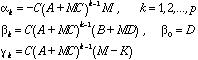
where M can be interpreted as a deadbeat observer gain, and under certain conditions, it becomes a steady-state Kalman filter gain.

Example 2: On the other hand, the coefficients of an ARMAX model

can be shown using observer Markov parameters that they are related to the state-space model coefficients by

where M can be interpreted as a deadbeat observer gain, and K is a steady-state Kalman filter gain. Using observer Markov parameters we can create many other kinds of input-output models (open-loop, closed-loop, forward-time, backward-time, deterministic, stochastic, one-step ahead, multi-step ahead, etc.) and know how the coefficients of each model are related to the system original state-space representation. See Phan et al. (April 1995) for more details.

• Generalized Cayley-Hamilton Theorem: The standard Cayley-Hamilton theorem states that a matrix satisfies its own characteristic equation where the coefficients of this characteristic polynomial are scalars. In the generalized Cayley-Hamilton case the "characteristic" polynomial of a matrix is defined with respect to itself and another (auxiliary) matrix, and the coefficients of such a generalized characteristic polynomial are matrices. In the case of state-space system identification, the output matrix C is such an auxiliary matrix. With this generalized Cayley-Hamilton theorem, one can prove such things as how multiple-output n-th order state-space model can be represented by a matrix input-output difference equation with order less than n (system identification), how the coefficients of an input-output model identified with disturbance-corrupted data are related to those of the disturbance-free model (system identification in the presence of unknown disturbances), how one can create input-output models where the disturbance effect can be totally explicit, totally implicit, or partially explicit and partially implicit (selective disturbance cancellation), how to design controllers for feedback stabilization and disturbance rejection (predictive control), among many other results. For more details, please refer to the publications by Goodzeit and Phan (1997) on the problems of system identification, disturbance identification, and disturbance rejection, and Phan, Lim, and Longman (1998) on the problem of predictive control.

System Identification for Predictive Control

Given a model of the system, one can use it to design a (model-based) controller. If a model is not available but a sufficient amount of input-output data is available, one can use the data to identify a model of the system first, and then use that identification model to design a controller. Each particular model-based controller design requires knowledge of certain combinations of system model parameters (say the system controllability matrix). Here we explore the idea of using identification theory to obtain directly what a particular controller design needs instead of first obtaining a model of the system from which the needed parameter combinations are computed. In this fashion we directly compute the controller gains from input-output data instead of working through an intermediate identified model. This situation is very much like what is known as direct adaptive control. The type of controllers that are most suitable for this approach of direct data-based controller synthesis is predictive control. On a very flexible and lightly damped systems with complex dynamics, we have been able to demonstrate that this direct approach produces controllers with higher performance than those derived from an intermediate identification model. For more information see Phan, Lim, and Longman (1998). If what a predictive controller needs is a multi-step ahead state estimator then it can be identified from input-output data as well. This solution is presented in Lim and Phan (1997). See also the general topic of Predictive Control.

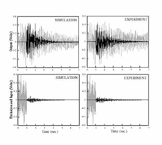
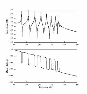
Illustration: The following figures illustrate the performance of a vibration suppression controller designed directly from a set of experimental input-output data. The design procedure bypasses the intermediate step of identifying a model of the system first. The right figures show the frequency response functions of a 10-rod configuration of SPINE. The system is very lightly damped and flexible, making it difficult to control. The left figures show a comparison between simulated and actual experimental results. The upper figures contain the system response with control (dark) and without control (light). The lower figures show the expected and actual control input signals. Close agreement between simulated and experimental results confirms the validity of the design approach.

   

System Identification in the Presence of Unknown Disturbances

The problem of state-space system identification in the presence of unknown disturbances is studied. We show that exact identification of a system disturbance-free dynamics is possible in the presence of completely unknown periodic disturbances. Provided the order of an assumed model is sufficiently large, the disturbance effect can be completely absorbed into the coefficients of an identified model that relates excitation input to disturbance-corrupted output. Interestingly, the details of the absorption are such that the system disturbance-free dynamics can still be recovered correctly from the identified disturbance-corrupted model as if there were no disturbances present. In addition to identifying the system disturbance-free dynamics correctly, the disturbance effect can also be extracted. From this information, we can obtain the steady-state contribution of the unknown disturbances on the output data, and a corresponding disturbance-cancellation feedforward control signal. The formulation only requires measurements of the control excitation inputs and the system disturbance-corrupted outputs. There is no need to measure the disturbances, or the disturbance-correlated signals, or to know their periods or profiles, or to use steady-state data. In addition, the disturbance periods need not be integer multiples of the sampling interval. Required to be known, however, are an upper bound on the (effective) order of the system dynamics and an upper bound on the number of disturbance frequencies. When implemented recursively, the developed method can handle systems whose dynamics and disturbance frequencies are slowly-time varying. The developed theory is suitable for multi-input, multi-output systems with single or multiple disturbance sources. In the case of unknown non-periodic disturbances, the problem of system and disturbance identification becomes ill-posed, but we show that it is still possible to obtain approximate but highly accurate identification results. The developed theory is verified by extensive simulation on realistic spacecraft models and experiments on a flexible structure testbed. For more details, see the publications by Goodzeit and Phan (1997) and also the general topic of Clear-Box Adaptive Control.

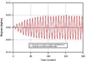
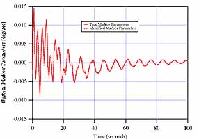
Illustration: The following figures illustrates how system identification can still be carried out correctly with disturbance-corrupted data. A high fidelity model of a communication satellite as shown above is used in this simulation. A periodic disturbance is injected into the satellite core, which corrupts the output response, while the system is randomly excited to collect data for system identification. The system responses with and without the disturbance presence are shown in the lower left figure. The disturbance effect is quite dominant: the much smaller signal is the system response without the disturbance and the much larger signal is the system response in the presence of the disturbance . Despite the severity of the disturbance, the system disturbance-free dynamics can still be identified correctly. The right figure shows a comparison between the identified versus true pulse responses of the satellite. This simulation was carried out to test the feasibility of using this identification technique on an actual spacecraft where the disturbance source itself cannot be turned off, and only disturbance-corrupted data is available for system identification.

  

System Identification for Clear-Box Intelligent Adaptive Control

It is shown that system identification can still be performed correctly with output data severely corrupted by unknown periodic disturbances. In addition to correct identification of the system disturbance-free dynamics, the disturbance contribution on the output can be identified correctly as well. This result leads to a new clear-box disturbance rejection scheme where -- prior to applying any control -- the contribution of each disturbance frequency on the system output and the corresponding control effort needed to cancel it can be determined. With this knowledge, informed decision can be made as to which disturbance frequencies should be canceled and which should be ignored before turning on the controller. This selective disturbance cancellation capability is particularly important when the disturbance sources, the output sensors, and the control actuators are all non-collocated, and only limited control energy is available. Experimental results are used to illustrate this new clear-box approach to disturbance rejection. Clear-box approach is contrasted to black-box approach where one finds out after the fact (e.g., actuator saturation). Extensive use of system identification allows one to exclude scenarios that would result in poor performance if the system attempts to cancel all disturbance frequencies. Instead, with this clear-box approach, one has a very good idea on the nature of the problem and the expected outcome given the actuator constraints before turning the control system on. The formulation only requires measurements of the control excitation inputs and the system disturbance-corrupted outputs. There is no need to measure the disturbances, or the disturbance-correlated signals, or to know their periods or profiles, or to use steady-state data. See the publications by Goodzeit and Phan (1997), Goodzeit, Phan, and Frueh (to appear), and Clear-Box Adaptive Control for more details.

Illustration: In this identification experiment of the T-Truss, random excitation is applied to the proof-mass control actuators located at one end of the structure. Acceleration measurements are made at one node on the other end of the structure. An "unknown" disturbance is injected into the structure while data is being collected for identification. This disturbance signal consists of 10 harmonic components, 5 of them are (by design) coincident with the system flexible modes. Only excitation input data and disturbance-corrupted output data are used for system identification which successfully recovers correctly the system disturbance-free input-output dynamics by separating overlapping system and "disturbance modes". All 10 disturbance frequencies are also correctly identified as shown in the table. In addition, the identification technique computes the contribution of each disturbance frequency on each of the two output accelerometers, and the control effort needed at each of the two control actuators to cancel each of these disturbance frequencies. All of this information is obtained by identification alone before any actual control is applied. This predictive table supplies information for a "clear-box" disturbance rejection system where only a certain number of disturbance frequencies should be intelligently selected for cancellation. This is often the case in difficult situations where the control actuators have limited capability, and the disturbance sources, sensors, and actuators are all non-collocated. Without this intelligent selection, a "black-box" adaptive control system would quickly saturates the available control resources.