Prediction of Quantum Process Evolution from Laboratory Data

A key to successful control of a quantum process is an understanding of how the manipulation of controlled laser pulse shape affects the final outcome (e.g., fraction of atoms or molecules occupying a particular quantum state). Certainly, such a prediction can be made if one can develop a detailed physical model of the process from first principles. In the course of developing such a model, however, certain idealized assumptions must be made about the quantum process itself or the laboratory environment. When dealing with complex systems, the developed analytical model is too imprecise for high-quality control. On the other hand, an identification model is extracted directly from laboratory data, and it is not susceptible to idealized assumptions of an analytical model. The real strength of an identification model is that it can be used effectively for the specific control application at hand. With a model that correctly describes and predicts how a change in the control action affects the final outcome, suitable adjustment to the controlled electric field can be made. Initial simulation studies on a simple quantum system by Phan and Rabitz (1997) suggests that this is potentially quite effective. A local identification model predicts the temporal evolution of the population occupying a particular state (an energetically degenerate upper level in this example) given a particular laser pulse shape. An inverse model predicts the necessary laser pulse shape given the desired evolution of the above mentioned population.

 

Illustration: The illustration is based on a simple four-level quantum mechanical system consisting of a ground level (level 1), a close lying excited level (level 2), and two energetically degenerate upper levels (levels 3 and 4). The objective of the problem is to drive the system from level 1 to level 4 in a prescribed amount of time. The measured output is the population of level 4. The system is driven by three constant amplitude laser pulses over the specified time interval, whose frequencies match those of the three transitions. The right figure shows an overlay of the actual output trajectory versus that predicted by the identified input-output model. The figure on the left shows a portion of the actual laser pulse shape and that represented in the identification model. This model correctly describes and predicts the relationship between the laser pulse shape and final outcome, and can be used as an effective aid in quantum control.

    

Self-Guided Learning Control of Quantum Processes

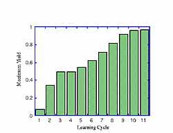
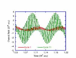
This work develops a self-guided algorithm for direct laboratory synthesis of controls to manipulate quantum-mechanical systems. The primary focus is on an algorithm that is based on the identification of a laboratory input-output map from a sequence of controls, and their observed impact on the quantum-mechanical system. This map is then employed in an iterative fashion, to sequentially home in on the desired objective. The objective may be a target quantum state at a final time, or a continuously weighted observational trajectory. The self-guided aspects of the algorithm are based on implementing cost functional that only contains laboratory-accessible information. Through choice of the weights in this functional, the algorithm can automatically stay within the bounds of each local input-output map, and indicate when a new map is necessary for additional iterative improvement. These concepts can be generalized to include the direct use of laboratory settings, rather than observation of the control itself. Simulation on a four-level quantum system is used to illustrate this learning algorithm. More details can be found in Phan and Rabitz (1999).

 

Illustration: A quantum mechanical system consisting of a ground level (level 1), a close lying excited level (level 2), and two energetically degenerate upper levels (levels 3 and 4) is used in this quantum control simulation. The objective of the problem is to drive the system from level 1 to level 4 in a prescribed amount of time. The measured output is the population of level 4. The system is driven by three constant amplitude laser pulses over the specified time interval, whose frequencies match those of the three transitions. Learning is carried out "from scratch" without any prior knowledge of the process dynamics. A sequence of intermediate desired trajectories (not shown explicitly in the figure) is successfully met by iterative trials designed from their respective input-output maps. During the entire process, input-output data used to identify the intermediate models for the next set of runs are obtained by perturbing the last learned values of the control coefficients from the previous set of runs. The left figure shows the transition eventually taking place with nearly perfect yield by iterative learning. The right figure shows a portion of the initial laser pulse shape versus that eventually obtained after learning.