System Identification with Identified Hankel Matrix
In many state-space identification techniques, the Hankel matrix appears rather often because a state-space model can be derived from its singular value decomposition (SVD). The Hankel matrix comprises of the Markov parameters arranged in a specific Toeplitz pattern. Much efforts have been placed on the problem of obtaining the Markov parameters from input-output data by time or frequency domain approaches. Once the Markov parameters are determined, they become entries in the Hankel matrix for state-space identification.
It can be proven that the rank of the Hankel matrix is the order of the system. With perfect noise-free data, the minimum order realization can be easily obtained by keeping only the non-zero Hankel singular values. With real or noise-contaminated data, one would hope for a significant drop in the singular values that signals the "true" order of the system, but while this can happen with low-noise simulated data, it rarely happens with real data. A reduced-order model obtained by retaining only "significant" singular values tends to be poor in accuracy. Indeed, this issue remains one of the most unsatisfactory discrepancy between what is expected in theory and what is actually observed in practice. One may argue that real systems are both non-linear and infinite dimensional. While this is certainly true in many cases it is not to blame in all cases. A common procedure is to keep all Hankel singular values at the expense of a high-dimensional state-space model, and use a separate post-identification procedure such as model reduction is to reduce the dimension of the identified model. However, any time model reduction is invoked, some accuracy is lost. It is preferable to have an identification method that produces a "true" or effective order model directly in the first place.
This work examines a strategy where the entire Hankel matrix itself is identified from input-output data. ARMarkov models appear naturally in this identification problem. Interestingly, we were able to show the new approach is effective in detecting the "true" or effective order of the system, hence it is capable of producing relatively low-dimensional state-space model. This work thus resolves the long standing discrepancy between what is expected in theory and what is actually observed in practice with regard to the rank of a Hankel matrix and its suggestion about the system "true" or effective order. More information can be found in Lim, Phan, and Longman (1998a).
Illustration: The first test uses a three-input three-output set of data collected from the Hubble Space Telescope (HST) in orbit. The system is operating in closed-loop, hence it is highly damped. For this reason the problem of order determination may be difficult. The HST has six gyros located on the optical telescope assembly which are used mainly to measure the motion of the primary mirror. The outputs are expressed in terms of the three angular rates in the vehicle coordinates. The input commands excite the telescope mirror and structure and they are given in terms of angular acceleration in the three rotational vehicle axes. The data record is 620 seconds long, and sampled at a relatively low rate of 10 Hz. The identification results are shown below for one output. The identified Hankel matrix approach produces a 3-mode model that reproduces the data quite accurately. This result is in agreement with that obtained with a more substantial set of data sampled at a higher resolution. The identified Hankel matrix approach is based on the Hankel-Toeplitz model which can be thought of as a family of ARMarkov models. Notice how the identified Hankel matrix approach produces a sharp drop in the prediction quality at the "correct" system order. This is exactly what one would like to see in practice.
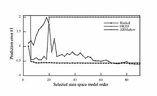
Illustration: This set of data is obtained from a two-input two-output truss developed for vibration control of flexible space structures at NASA Langley Research Center. The inverted L-shape structure consists of nine bays on its vertical section, and one bay on its horizontal section, extending 90 inches and 20 inches respectively. The shorter section is clamped to a steel plate which is rigidly attached to the wall. At the tip of the truss are two cold air jet thrusters, and two accelerometers. For identification, the structure is excited using random inputs to both thrusters. The data record is 8 seconds long and is sampled at 250Hz. This data record is relatively short and the system is more difficult to be identified because it has a small number of dominant modes and a large number of less dominant but still significant modes. Again, the identified Hankel method produces the smallest order model that is comparable in accuracy to a much higher order OKID model. Notice again how the identified Hankel matrix produces a drop in the prediction quality at the "correct" system order and then the curve flattens out.
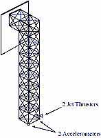
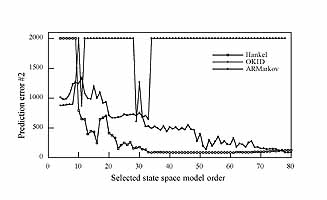
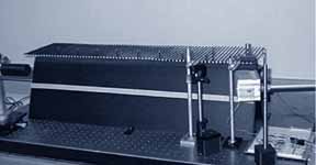
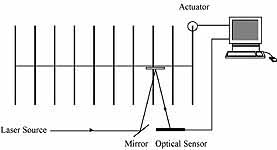
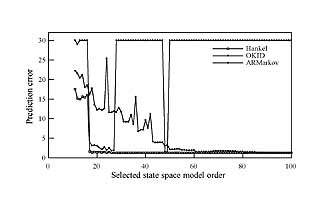
Illustration: The third set of single-input single-output data is obtained from a compact yet very lightly damped and flexible apparatus. SPINE consists of a series of parallel steel rods mounted on a thin center wire. In its 10-rod configuration, an actuator controls the vertical position of the tip of the first rod. A laser-based optical sensing system detects the torsional motion of the third rod, and the tenth rod is clamped to a rigid support. Since the tip of the first rod is a controlled input and the last rod is fixed, the "effective" order of the system is expected to be around 16 (for 8 flexible modes). With this set of data we have an opportunity to see if the method produces a state-space model of this expected order. The system is excited by a random input for 80 seconds and the resultant output is recorded at a sampling rate of 200 Hz. Obseve that the prediction error drops sharply and then flattens out at the expected order of 16 for the identified Hankel method. Again the ideal pattern is observed for this set of data.
Optimal State Estimation with ARMarkov Models
State estimation is an important element of modern control theory. Given a known model of the system under the influence of process and measurement noise with known statistics specified in terms of their covariances, it is well known that the Kalman filter is an optimal state estimator in the sense that its state estimation error is minimized. In practice, it may be difficult to design such an optimal estimator because neither the system nor the noise statistics can be known exactly. From the point of view of system identification, information about the system and the noise statistics are embedded in a sufficiently long set of input-output data. Thus it would be advantageous to be able to obtain such an estimator directly from input-output data without having to identify the system and the noise statistics separately. This is the problem of observer identification. In this work, we show how a state estimator can be identified directly from input-output data using ARMarkov models.
In fact, it is also possible to identify a state-space model together with an observer gain using other kinds of models such as ARX and ARMAX. But with these techniques it is not always possible to determine the order of the state space realization by Hankel singular value truncation alone and a separate post-identification model reduction procedure must be used. With ARMarkov models, we have the opportunity to identify state estimators with true or effective orders without having to invoke a separate model reduction step as normally required. More information can be found in Lim, Phan, and Longman (1998b).
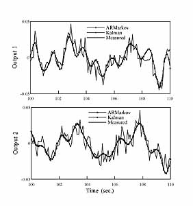
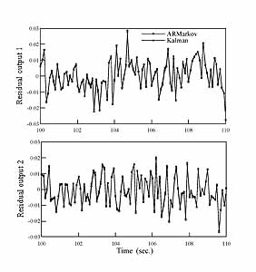
Illustration: Consider a chain of three masses connected by springs and dampers with force input to the first mass and position measurements of the last two masses. The system is excited by random input, and the output data is corrupted by significant process and measurement noise. Because this is a simulation, we can actually compute the noise statistics in terms of their covariances. From exact knowledge of the system and the computed process and measurement noise covariances, a Kalman filter is designed. The Kalman filter represents the "best" or optimal estimation that can be achieved for the given system with the known noise statistics. This is the optimal result against which our identified state estimator will be compared. Next, from the above set of noise corrupted input-output data alone, a state estimator is identified, and this is done without knowledge of the system and without knowledge of the embedded process and measurement noise statistics. We then compare the quality of the identified state estimator with that of the optimal Kalman filter. The left figures show the actual measured (noise-corrupted) outputs together with an overlay of the results of the optimal Kalman filter estimation and the identified 6-th order state estimator. The jagged curves are the measured noise-corrupted outputs. The smooth curves represent the optimal filtering by the Kalman filter. The results obtained with the identified state estimator practically match the Kalman filter result (there are two nearly overlapping smooth curves in each of the two left figures). The right figures show a comparison of the residuals themselves, for each of the two outputs. Recall that the Kalman filter is derived with exact knowledge of the system and noise statistics, whereas the identified state estimator is derived from input-output data alone. Any difference between these two residuals is hardly distinguishable because they practically overlap in these figures. Thus this simulation confirms that our identified state estimator is indeed optimal. This kind of verification can only be carried out with simulation data (not with experimental data) because we need to know both the plant model and the noise statistics exactly to determine the expected optimal estimation results.